- dilks's home page
- Posts
- 2019
- 2018
- December (1)
- November (1)
- October (1)
- August (2)
- July (4)
- June (3)
- May (1)
- April (2)
- March (2)
- February (1)
- January (5)
- 2017
- December (3)
- November (1)
- October (2)
- September (3)
- August (2)
- July (2)
- June (1)
- May (2)
- March (3)
- February (3)
- January (3)
- 2016
- November (2)
- September (4)
- August (2)
- July (6)
- June (2)
- May (3)
- April (1)
- March (2)
- February (3)
- January (2)
- 2015
- December (3)
- October (3)
- September (2)
- August (6)
- June (3)
- May (3)
- April (4)
- March (3)
- February (5)
- January (3)
- 2014
- December (1)
- November (1)
- October (3)
- September (4)
- August (3)
- July (3)
- June (2)
- May (2)
- April (2)
- March (1)
- 2013
- 2012
- 2011
- My blog
- Post new blog entry
- All blogs
Run 15 PMT Gain Curves
GAIN CURVE FITTING
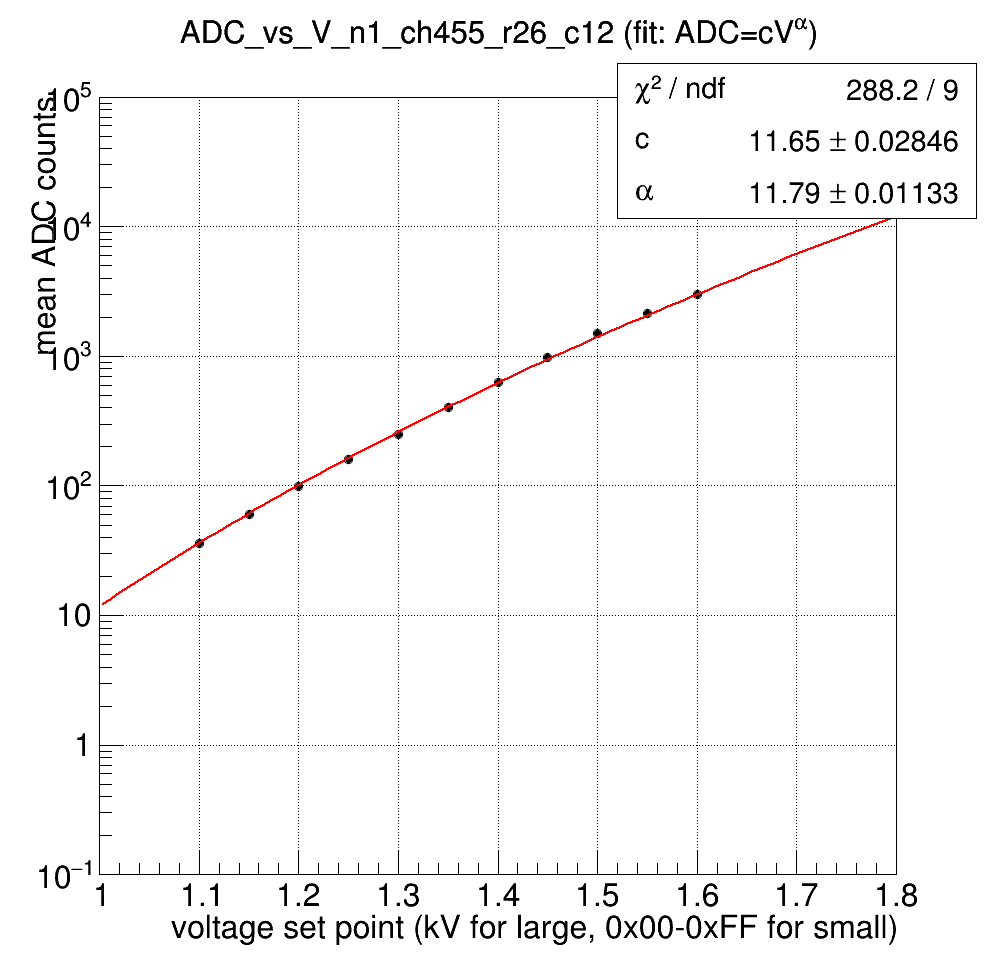
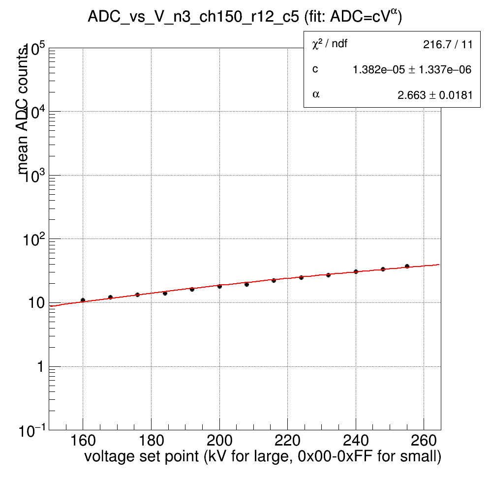
For each cell, the ADC distribtution for each HV setpoint was fit to a Gaussian function; subsequently, the extracted ADC means were plotted against HV setpoints and fit to the function ADC=cVα, where V is the setpoint, and c and α are fit parameters. The fit results (from Day21) are contained in the following directory:
Note: points outside the range 10 < mean ADC < 3800 were dropped from the fits and the graphs, since we often saw saturation at ADC ~4000 (not 4096 because of some cases where the pedestal was shifted.. 3800 seemed like a "safe" upper limit after looking to fix as many chisquare outliers as possible)
=====================================================================================
DAY 41 DATA
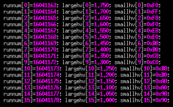
NOTE: Lecroy Crate 7008 had problems and was disabled for these runs!
run numbers and HV setpoints table:
.png) Lecroy crate 7008 was disabled
Lecroy crate 7008 was disabled
.png)


=====================================================================================
DAY 21 DATA
On day 21, we took 13 runs with the following HV setpoints:
[runnum] [large cell (kV)] [small cell (0x00-0xFF)]
16021065 1.10 0xA0
16021066 1.15 0xA8
16021067 1.20 0xB0
16021068 1.25 0xB8
16021069 1.30 0xC0
16021070 1.35 0xC8
16021071 1.40 0xD0
16021072 1.45 0xD8
16021073 1.50 0xE0
16021074 1.55 0xE8
16021075 1.60 0xF0
16021076 1.65 0xF8
16021077 1.70 0xFF
These data were acquired while the STAR magnet was on
200 events were recorded per run
Figure 1:
Here are examples of typical gain curves (large cell on left, small cell on right)
Here are the fit parameters for the FMS; note that the north-top quadrant is currently incomplete (upper-left corner)
Figure 2:
.png)
Figure 3:
.png)
Figure 4:
.png)
Figure 5:
.png)
Figure 6:
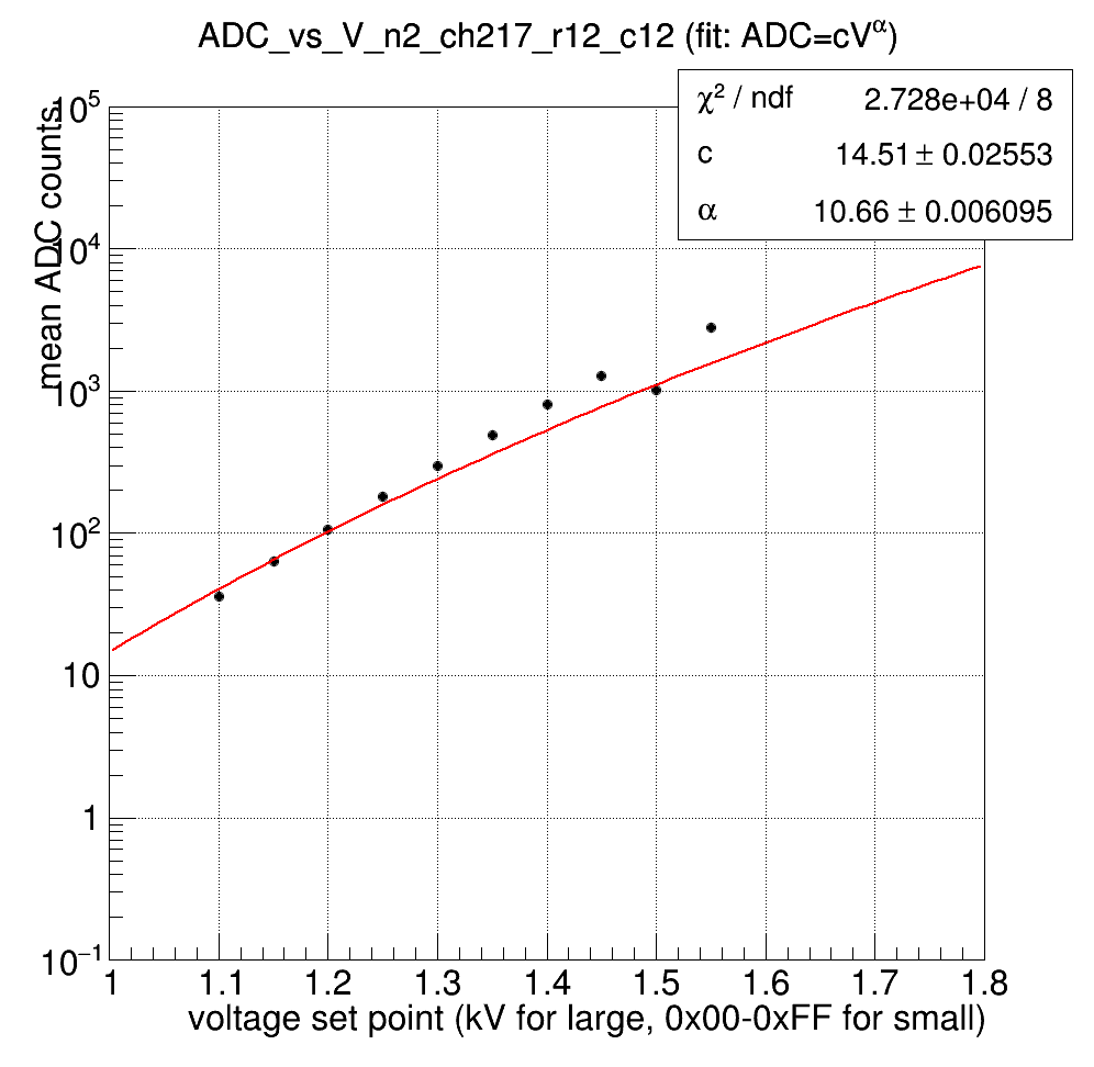
chisq/ndf for each fit; anomalously high chisquares are cases where 1 point deviated downward from the fit line (see figure 8)
.png)
Figure 7:
chisq for each fit; anomalously high chisquares are cases where 1 point deviated downward from the fit line (see figure 8)
.png)
Figure 8:
Most of the fits are good; an example gain curve with a high chisq is shown below. One point at 1500 V is causing the fit problem. All other channels that had high chisq fits were also cases where 1 point had lower ADC counts then the local trend line.
AVERAGE FIT PARAMETERS
We now classify sets of channels and compute the average fit parameters for these sets. Figure 8 shows the classification:
Figure 9:
Classification of channel types (locations of channels on left; bar chart for number of channels on right)
GREEN = large regular
CYAN = large outer edge
YELLOW = small russian
RED = small yale

.png)
Figure 10:
α distribution for large "regular" cells (left) and large edge cells (right)

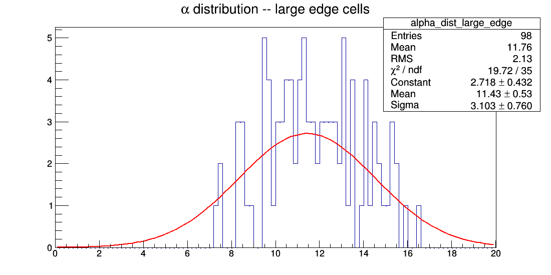
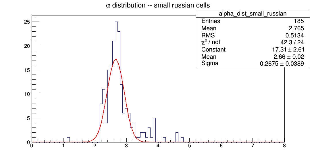
Figure 11:
α distribution for small cells with Russian PMTs/bases (left) and those with Yale PMTs/bases (right)

- dilks's blog
- Login or register to post comments
