- jwebb's home page
- Posts
- 2019
- 2018
- 2017
- 2016
- 2015
- 2014
- 2013
- November (1)
- October (1)
- September (1)
- July (1)
- June (1)
- April (1)
- March (3)
- February (1)
- January (1)
- 2012
- 2011
- December (2)
- September (3)
- August (5)
- July (6)
- June (6)
- May (1)
- April (5)
- March (5)
- February (2)
- January (2)
- 2010
- December (3)
- October (3)
- September (2)
- August (2)
- June (2)
- May (4)
- April (4)
- March (2)
- February (4)
- January (10)
- 2009
- 2008
- 2007
- 2006
- July (1)
- My blog
- Post new blog entry
- All blogs
Data / MC comparisons for isolation cut
1.0 Absolute Normalization for Histograms
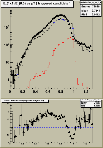
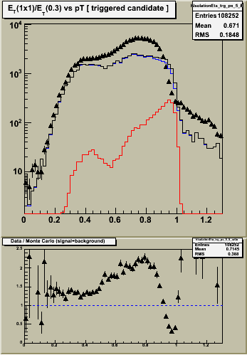
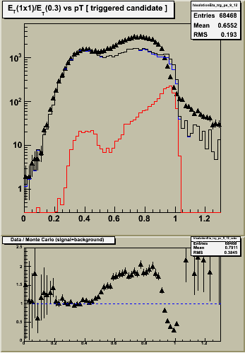
Notes:
0. Data sample: runs from pp2006 longitudinal after L2gamma trigger thresholds stabalized (ID = 137641)
1. Pythia's absolute normalization is used to create figure 1.
2. A pT cut of 5.2 Gev has been imposed on both data and Monte Carlo.
3. The only other cuts which are applied are (1) the event satisfied the L2gamma trigger (ID = 137641)
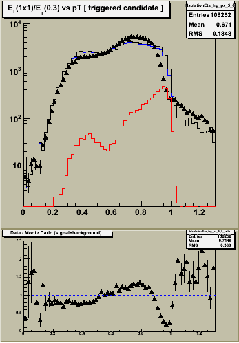
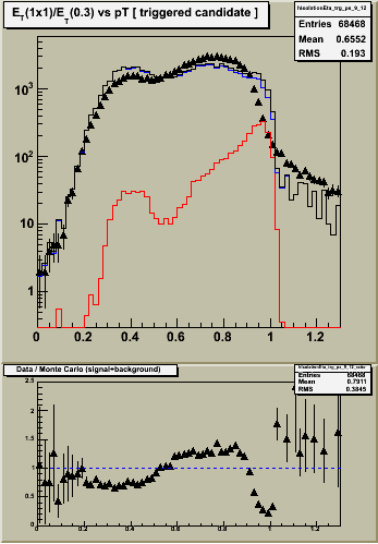
4. The agreement between data and MC is poor right where we need it to be good at RI ~ 1, where the photons are. The origin of this effect is probably related to the sampling fraction problem... smaller energy deposits require a larger "fudge" factor to get the thrown energy back.
5. Data and MC agree "well" (in shape if not normalization) in the region of RI < 0.5, for etabins 5-12.
- There is a peak in the data, reproduced by the MC spectra, around RI ~ 0.4.
- This peak originates from photons which convert having the energy of the e+ and/or e- counted once in the numerator (the calorimeter tower), and multiple counted in the denominator (the e+ and/or e- track pT plus the calormiter ET).
- We cannot make a definitive statement about the normalization of this peak because
- Pythia cross section is not NLO (its not even LO)
- We do not know if TPC tracking efficiency or resolution is well modeled here, and
- The amount of material in front of the endcap is somewhat uncertain.
- The flat shape suggests that the distribution of material in front of the EEMC is described well. However, the normalization changes from outer four etabins to middle four etabins. Suggests either excess or deficiet of material in front of these areas.
2.0 Common Yield Normalization
In figure 2 below, scale the MC histograms so that the data and jet+prompt distributions have equal counts.
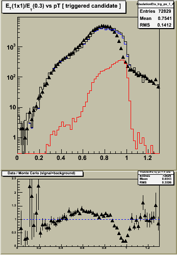
Notes:
1. Things look "better" with common normalization. Discrepancies between data and MC are reduced to the ~20% level for RI<0.8. Of course, its still quite awful where it needs to be good.
2. With this normalization we see the same level of discrepancy in all three eta ranges for RI < 0.8. Details / statistics change, but the magnitude of the discrepancy remains the same.
3.0 Plans
- jwebb's blog
- Login or register to post comments
